Yarra Water Analysis

Overview

The YarraWaterAnalysis package provides tools for analyzing and visualizing streamflow data from the Yarra River at McMahons monitoring site.

Load the YarraWaterAnalysis package using the library() function.

library(YarraWaterAnalysis)

Built-in data description

The package includes daily mean streamflow data with the following key variables:

#> Warning in attr(x, "align"): 'xfun::attr()' is deprecated.
#> Use 'xfun::attr2()' instead.
#> See help("Deprecated")
#> Warning in attr(x, "align"): 'xfun::attr()' is deprecated.
#> Use 'xfun::attr2()' instead.
#> See help("Deprecated")

YARRA WATER DATA
Variable	Type	Description
site_id	double	Site Id
site_name	character	Site Name
datetime	double	Datetime yyyy-mm-dd hh:mm:ss
data_type	character	Data type
parameter_id	double	Parameter id
parameter	character	Parameter
value	double	Daily mean streamflow in ML/day
unit	character	Unit
quality	double	Quality
resolution	character	Resolution
date	double	Date of measurement
year	double	Year
month	integer	Month
day	integer	Day
season	character	Seasonal classification
flow_category	character	Flow magnitude category
log_flow	double	Log Flow
flow_7day_avg	double	Flow 7day avg

Calculate Flow Statistics

calculate_flow_stats(yarra_water_data)

You can use this function to calculate basic statistics for Yarra River streamflow data

analyze_seasonal_patterns

# Analyze seasonal patterns
seasonal_stats <- analyze_seasonal_patterns(yarra_water_data)
print(seasonal_stats)
#> # A tibble: 4 × 6
#>   season avg_flow median_flow max_flow min_flow n_observations
#>   <chr>     <dbl>       <dbl>    <dbl>    <dbl>          <int>
#> 1 Autumn     248.          75    14085        0           3347
#> 2 Summer     272.         102     6131        0           3535
#> 3 Winter     922.         283    17245        0           3407
#> 4 Spring    1023.         366    18687        0           3823

# Plot seasonal distribution
ggplot(yarra_water_data, aes(x = season, y = value, fill = season)) +
  geom_boxplot() +
  labs(title = "Yarra River Flow by Season",
       x = "Season", y = "Flow (ML/day)") +
  theme_minimal()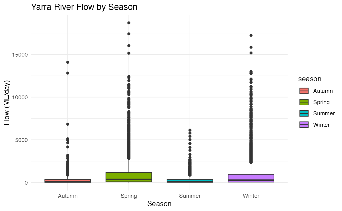

You can use this function to analyze seasonal patterns

detect_high_flow_events

#> # A tibble: 6 × 18
#>   site_id site_name   datetime            data_type parameter_id parameter value
#>     <dbl> <chr>       <dttm>              <chr>            <dbl> <chr>     <dbl>
#> 1  229143 YARRA @ CH… 1975-10-26 23:59:59 Quantity          142. Streamfl… 18687
#> 2  229142 YARRA @ TE… 1975-10-26 23:59:59 Quantity          142. Streamfl… 17399
#> 3  229143 YARRA @ CH… 1977-07-01 23:59:59 Quantity          142. Streamfl… 17245
#> 4  229143 YARRA @ CH… 1975-10-27 23:59:59 Quantity          142. Streamfl… 16014
#> 5  229143 YARRA @ CH… 1977-06-20 23:59:59 Quantity          142. Streamfl… 15849
#> 6  229143 YARRA @ CH… 1977-06-19 23:59:59 Quantity          142. Streamfl… 15164
#> # ℹ 11 more variables: unit <chr>, quality <dbl>, resolution <chr>,
#> #   date <date>, year <dbl>, month <ord>, day <int>, season <chr>,
#> #   flow_category <chr>, log_flow <dbl>, flow_7day_avg <dbl>

You can use this function to detect high flow event

Interactive Exploration

Launch the Shiny application for interactive data exploration:

# Launch the interactive app
# launch_app()

The Shiny app provides: